Python ‘virtual environment’ to integrate scVI with Seurat

Multiomics

Biology

A short

Author

Rishi Das Roy

Published

October 13, 2025

This post provides alternative of the conda environment to use scVI-tools through Seurat wrappers. For the R users (and not expert in python), SeuratWrappers provides scVIIntegration method which is really useful and explained here. However, this depends on conda environment which may not be available on every platform, like some HPCs I use.

Here I discuss how to use python’s virtual environment and its own challenges. The hurdles are

Create virtual environment
- R commands to create python virtual environments.
- The default command will install dependency numpy version > 2 which does not work with scVI-tools and will throw internal errors.
Rewrite the scVIIntegration function.

The required packages

library(Seurat, quietly = TRUE, verbose = FALSE)
library(SeuratData, quietly = TRUE, verbose = FALSE)
library(SeuratWrappers, quietly = TRUE, verbose = FALSE)
library(ggplot2, quietly = TRUE, verbose = FALSE)
library(patchwork, quietly = TRUE, verbose = FALSE)
options(future.globals.maxSize = 1e9)
library(reticulate, quietly = TRUE, verbose = FALSE)

1 Installation

Declare a path to install the python packages and use following commands of reticulate package. The downloaded files are could be very big and it is useful to declare the cache-dir for smooth installation

install_dirPath <- "/your/path_to/install/"
 
reticulate::virtualenv_create(envname = install_dirPath, force = TRUE,
                              version = ">=3.11", packages = c("numpy<2"),
                              pip_options = c("--cache-dir=/your/path_to/tmp/"))
reticulate::virtualenv_install(envname = install_dirPath, 
                               packages = c("scvi-tools"), 
                               pip_version = FALSE,
                               pip_options = c("--cache-dir=/your/path_to/tmp/"))

Verify the numpy version?

reticulate::use_virtualenv(virtualenv=install_dirPath)
config <- py_config()
config$numpy$version

[1] '1.26.4'

2 Rewrite the scVIIntegration

The environment option is hard coded in the original function. Therefore, it needs to be redefined as below. Can you identify the line numbers to see the difference?

venv_scVIIntegration <- function (object, features = NULL, layers = "counts", venv_env = NULL, 
  new.reduction = "integrated.dr", ndims = 30, nlayers = 2, 
  gene_likelihood = "nb", max_epochs = NULL, ...) 
{
  reticulate::use_virtualenv(virtualenv = venv_env, required = TRUE)
  sc <- reticulate::import("scanpy", convert = FALSE)
  scvi <- reticulate::import("scvi", convert = FALSE)
  anndata <- reticulate::import("anndata", convert = FALSE)
  scipy <- reticulate::import("scipy", convert = FALSE)
  if (is.null(max_epochs)) {
    max_epochs <- reticulate::r_to_py(max_epochs)
  }
  else {
    max_epochs <- as.integer(max_epochs)
  }
  batches <- .FindBatches(object, layers = layers)
  object <- JoinLayers(object = object, layers = "counts")
  adata <- sc$AnnData(X = scipy$sparse$csr_matrix(Matrix::t(LayerData(object, 
    layer = "counts")[features, ])), obs = batches, var = object[[]][features, 
    ])
  scvi$model$SCVI$setup_anndata(adata, batch_key = "batch")
  model <- scvi$model$SCVI(adata = adata, n_latent = as.integer(x = ndims), 
    n_layers = as.integer(x = nlayers), gene_likelihood = gene_likelihood)
  model$train(max_epochs = max_epochs)
  latent <- model$get_latent_representation()
  latent <- as.matrix(latent)
  rownames(latent) <- reticulate::py_to_r(adata$obs$index$values)
  colnames(latent) <- paste0(new.reduction, "_", 1:ncol(latent))
  suppressWarnings(latent.dr <- CreateDimReducObject(embeddings = latent, 
    key = new.reduction))
  output.list <- list(latent.dr)
  names(output.list) <- new.reduction
  return(output.list)
}

Additionally, we have to make this function .FindBatches which is not exported by the SeuratWrappers for external uses.

Code

.FindBatches <- function(object, layers) {
  # if an `SCTAssay` is passed in it's expected that the transformation
  # was run on each batch individually and then merged so we can use
  # the model identifier to split our batches
  if (inherits(object, what = "SCTAssay")) {
    # build an empty data.frame indexed
    # on the cell identifiers from `object`
    batch.df <- SeuratObject::EmptyDF(n = ncol(object))
    row.names(batch.df) <- Cells(object)
    # for each
    for (sct.model in levels(object)) {
      cell.identifiers <- Cells(object, layer = sct.model)
      batch.df[cell.identifiers, "batch"] <- sct.model
    }
    # otherwise batches can be split using `object`'s layers
  } else {
    # build a LogMap indicating which layer each cell is from
    layer.masks <- slot(object, name = "cells")[, layers]
    # get a named vector mapping each cell to its respective layer
    layer.map <- labels(
      layer.masks,
      values = Cells(object, layer = layers)
    )
    # wrap the vector up in a data.frame
    batch.df <- as.data.frame(layer.map)
    names(batch.df) <- "batch"
  }

  return(batch.df)
}

3 Reproduce

The example given in the documentation of scVIIntegration.

# load in the pbmc systematic comparative analysis dataset
obj <- LoadData("pbmcsca")
obj[["RNA"]] <- split(obj[["RNA"]], f = obj$Method)
obj <- NormalizeData(obj)
obj <- FindVariableFeatures(obj)
obj <- ScaleData(obj)
obj <- RunPCA(obj)
obj

An object of class Seurat 
33694 features across 31021 samples within 1 assay 
Active assay: RNA (33694 features, 2000 variable features)
 19 layers present: counts.Smart-seq2, counts.CEL-Seq2, counts.10x_Chromium_v2_A, counts.10x_Chromium_v2_B, counts.10x_Chromium_v3, counts.Drop-seq, counts.Seq-Well, counts.inDrops, counts.10x_Chromium_v2, data.Smart-seq2, data.CEL-Seq2, data.10x_Chromium_v2_A, data.10x_Chromium_v2_B, data.10x_Chromium_v3, data.Drop-seq, data.Seq-Well, data.inDrops, data.10x_Chromium_v2, scale.data
 1 dimensional reduction calculated: pca

obj <- IntegrateLayers(
  object = obj, method = venv_scVIIntegration,
  new.reduction = "integrated.scvi",
  venv_env = install_dirPath,
  orig.reduction = "pca",  verbose = FALSE
)


Training:   0%|          | 0/258 [00:00<?, ?it/s]
Epoch 1/258:   0%|          | 0/258 [00:00<?, ?it/s]

obj <- FindNeighbors(obj, reduction = "integrated.scvi", dims = 1:30, verbose = FALSE)
obj <- FindClusters(obj, resolution = 2, cluster.name = "scvi_clusters", verbose = FALSE)

obj <- RunUMAP(obj, reduction = "integrated.scvi", dims = 1:30, 
               reduction.name = "umap.scvi", verbose = FALSE)
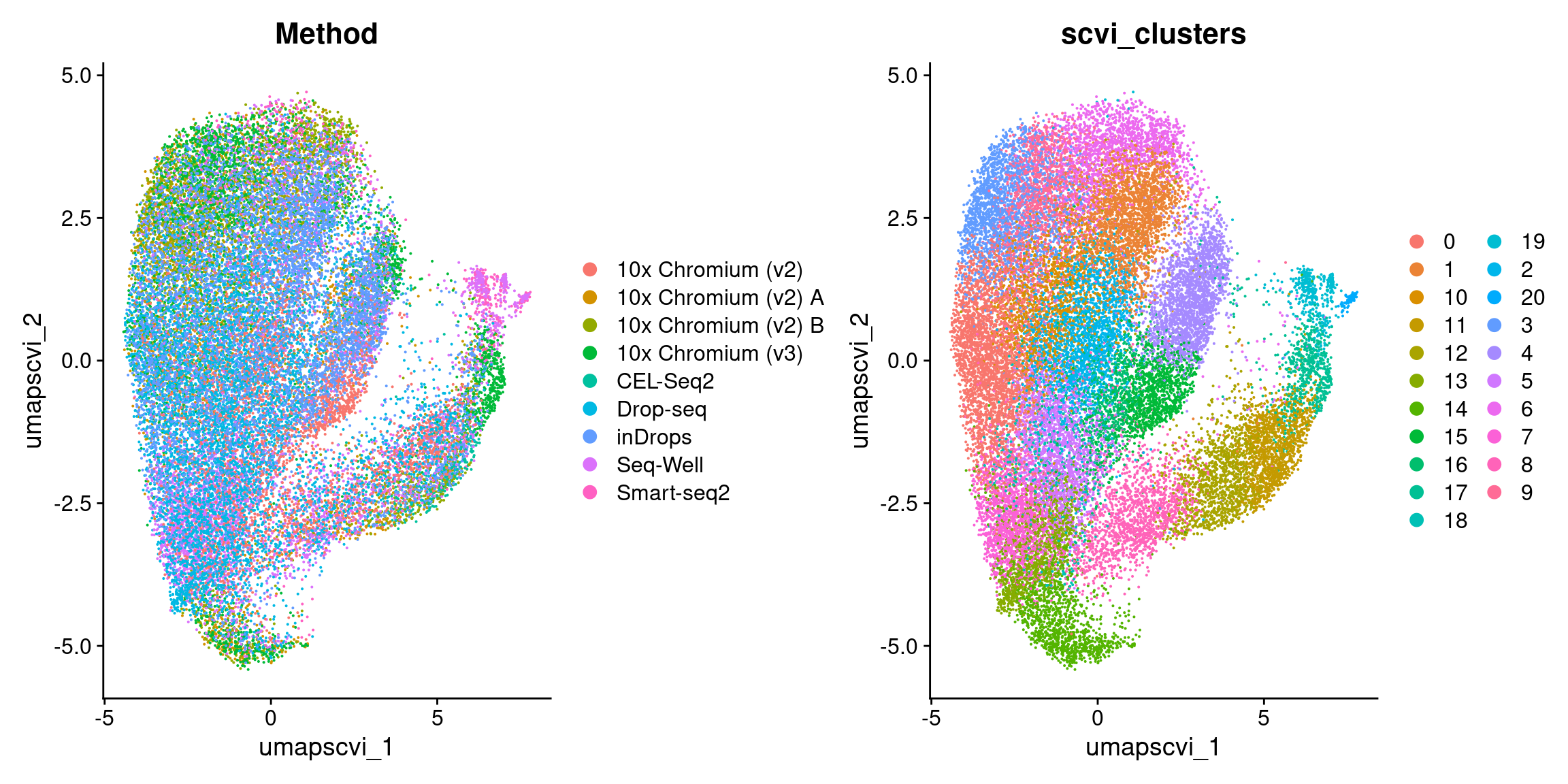
DimPlot(
  obj,
  reduction = "umap.scvi",
  group.by = c("Method", "predicted.celltype.l2", "scvi_clusters"),
  combine = TRUE, label.size = 2
)

sessionInfo

sessionInfo()

R version 4.4.0 (2024-04-24)
Platform: x86_64-pc-linux-gnu
Running under: Rocky Linux 8.9 (Green Obsidian)

Matrix products: default
BLAS/LAPACK: /opt/intel/oneapi/mkl/2024.1/lib/libmkl_gf_lp64.so.2;  LAPACK version 3.11.0

locale:
 [1] LC_CTYPE=en_US.UTF-8       LC_NUMERIC=C              
 [3] LC_TIME=en_US.UTF-8        LC_COLLATE=en_US.UTF-8    
 [5] LC_MONETARY=en_US.UTF-8    LC_MESSAGES=en_US.UTF-8   
 [7] LC_PAPER=en_US.UTF-8       LC_NAME=C                 
 [9] LC_ADDRESS=C               LC_TELEPHONE=C            
[11] LC_MEASUREMENT=en_US.UTF-8 LC_IDENTIFICATION=C       

time zone: Europe/Helsinki
tzcode source: system (glibc)

attached base packages:
[1] stats     graphics  grDevices utils     datasets  methods   base     

other attached packages:
 [1] reticulate_1.36.1        patchwork_1.2.0          ggplot2_3.5.1           
 [4] SeuratWrappers_0.3.5     pbmcsca.SeuratData_3.0.0 pbmcref.SeuratData_1.0.0
 [7] SeuratData_0.2.2.9001    Seurat_5.1.0             SeuratObject_5.0.2      
[10] sp_2.1-4                

loaded via a namespace (and not attached):
  [1] RColorBrewer_1.1-3     rstudioapi_0.16.0      jsonlite_1.8.8        
  [4] magrittr_2.0.3         spatstat.utils_3.0-4   farver_2.1.2          
  [7] rmarkdown_2.27         vctrs_0.6.5            ROCR_1.0-11           
 [10] spatstat.explore_3.2-7 htmltools_0.5.8.1      sctransform_0.4.1     
 [13] parallelly_1.37.1      KernSmooth_2.23-22     htmlwidgets_1.6.4     
 [16] ica_1.0-3              plyr_1.8.9             plotly_4.10.4         
 [19] zoo_1.8-12             igraph_2.0.3           mime_0.12             
 [22] lifecycle_1.0.4        pkgconfig_2.0.3        rsvd_1.0.5            
 [25] Matrix_1.7-0           R6_2.5.1               fastmap_1.2.0         
 [28] fitdistrplus_1.1-11    future_1.33.2          shiny_1.8.1.1         
 [31] digest_0.6.35          colorspace_2.1-0       tensor_1.5            
 [34] RSpectra_0.16-1        irlba_2.3.5.1          labeling_0.4.3        
 [37] unixtools_0.1-1        progressr_0.14.0       fansi_1.0.6           
 [40] spatstat.sparse_3.0-3  httr_1.4.7             polyclip_1.10-6       
 [43] abind_1.4-5            compiler_4.4.0         remotes_2.5.0         
 [46] withr_3.0.0            fastDummies_1.7.3      R.utils_2.12.3        
 [49] MASS_7.3-60.2          rappdirs_0.3.3         tools_4.4.0           
 [52] lmtest_0.9-40          httpuv_1.6.15          future.apply_1.11.2   
 [55] goftest_1.2-3          R.oo_1.26.0            glue_1.7.0            
 [58] nlme_3.1-164           promises_1.3.0         grid_4.4.0            
 [61] Rtsne_0.17             cluster_2.1.6          reshape2_1.4.4        
 [64] generics_0.1.3         gtable_0.3.5           spatstat.data_3.0-4   
 [67] R.methodsS3_1.8.2      tidyr_1.3.1            data.table_1.15.4     
 [70] utf8_1.2.4             spatstat.geom_3.2-9    RcppAnnoy_0.0.22      
 [73] ggrepel_0.9.5          RANN_2.6.1             pillar_1.9.0          
 [76] stringr_1.5.1          spam_2.10-0            RcppHNSW_0.6.0        
 [79] later_1.3.2            splines_4.4.0          dplyr_1.1.4           
 [82] lattice_0.22-6         survival_3.5-8         deldir_2.0-4          
 [85] tidyselect_1.2.1       miniUI_0.1.1.1         pbapply_1.7-2         
 [88] knitr_1.46             gridExtra_2.3          scattermore_1.2       
 [91] xfun_0.44              matrixStats_1.3.0      stringi_1.8.4         
 [94] lazyeval_0.2.2         yaml_2.3.8             evaluate_0.23         
 [97] codetools_0.2-20       tibble_3.2.1           BiocManager_1.30.23   
[100] cli_3.6.2              uwot_0.2.2             xtable_1.8-4          
[103] munsell_0.5.1          Rcpp_1.0.12            globals_0.16.3        
[106] spatstat.random_3.2-3  png_0.1-8              parallel_4.4.0        
[109] dotCall64_1.1-1        listenv_0.9.1          viridisLite_0.4.2     
[112] scales_1.3.0           ggridges_0.5.6         leiden_0.4.3.1        
[115] purrr_1.0.2            crayon_1.5.2           rlang_1.1.3           
[118] cowplot_1.1.3